Spectrum parameters

The basic task accomplished by FAST is to compute the absorption spectrum $P(\omega)$ of a molecular, i.e. finite system at a set of frequencies $\omega$ in some user-defined interval $\left[ \omega_{\hbox{\scriptsize min} },\omega_{\hbox{\scriptsize max} } \right]$. Such a spectrum is not in itself very useful since it is a set of discrete resonances with width and heights dependent on the regularisation parameter $\epsilon$. Paper 3 therefore describes an adaptative algorithm to extract transition frequencies, $\Omega_I$, and oscillator strengths, $f_I$, from the raw polarisability spectrum calculated by FAST. The algorithm proceeds by a two-tier iteration.

In the top level iteration, (i) the number of frequency points used (and polarisabilities, $P(\omega)$ computed, beware the cost in CPU time), is increased by a constant fraction; or (ii) the regularisation parameter $\epsilon$ is reduced by a step towards its target value; or (iii) both changes are made. In between top level iterations, the lower level iteration bears on the distribution of the frequency points. It uses the current spectrum to cluster the frequency points around the resonances, which improves the estimates of the a sum of Lorentzians to the spectrum.

Tier-two clustering is iterated until the resonance parameters $\Omega_I$ and $f_I$ are stable, after which tier-one update of the number of frequency points and the regularisation parameter, or both, are updated, and the cycle continues until convergence of the resonances between iterations. A combination of keywords provided at the end of this section can be used to invoke only tier two iterations.

The following parameters control the frequencies where FAST computes the optical polarizability $P(\omega)$, and how the adaptive algorithm described in paper 3 extracts the transition frequencies and oscillator strengths.

omega_min

(real): Lower bound of the frequency range.

Default: 0.02 in io_units

omega_max

(real): Upper bound of the frequency range.

Default: 0.4 in io_units

N.B. The default values of omega_min and omega_max are suitable for the visible spectral region if io_units are Rydbergs.

eps_units

(string): Units for the regularisation parameter $\varepsilon$.

Allowed values : Rydberg, cm-1, Angstrom, Hartree, nm, eV.

Default: Rydberg

freq_eps

(real): Regularization parameter $\epsilon$ in the response function which defines the apparent width of the resonances, cf.papers 1-3.

A positive value of freq_eps is interpreted as the target value towards which $\epsilon$ will be decreased during tier-one iterations of the adaptive algorithm. Making it small helps to identify resonances and specially to distinguish close resonances. But note that the linear response problem solved here describes undamped resonances ( no relaxation, coupling to phonons, etc.). Therefore, resonances are in principle infinite, whence the presence of the regularisation parameter in the equations, to 'pseudo-damp' them to finite height. Thus, if $\epsilon$ is too small, the linear system to be solved by GMRES tends to singularity when a frequency point happens to lie less than a few $\epsilon$ from a transition, producing numerical instabilities, such as failure of GMRES to converge, or unphysical solutions, such as negative polarisabilities.

When choosing freq_eps, users should bear in mind that the fit procedure pin-points transitions much more accurately than the width of the resonances ($\epsilon$), in the authors' experience typically to a precision of at least $\epsilon /100$.

File input_outputFileName_OddFrequency.txt provides a list of all frequencies which gave rise to a singular matrix.

A negative value of freq_eps causes FAST to deduce this parameter from the number of frequencies according to

$$freq\_eps = \frac{ 3*(omega\_max- omega\_min)}{2(nff-1)}$$

.

Default: $+0.01$Rydberg

nff

(integer):

A positive value of nff defines the initial number of frequency points at which to compute the spectra. The initial distribution of points is uniform in the target window $[\omega_{min},\omega_{max}]$ :

$$\omega_i = omega\_min + \frac{omega\_max- omega\_min}{nff-1 } (i-1) \mbox { with }i=1..nff$$

A negative value of nff causes the number of points to be controlled by the target regularisation parameter :

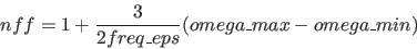$$nff = 1 + \frac{3}{2 freq\_eps}( omega\_max- omega\_min)$$ (1)

Default: $+257$

distribution

(string): The type of distribution used to compute the spectra. uniform for uniform distribution, and adaptive for non uniform distribution. In this case, the points will be localized near the peaks in the spectrum

Default: adaptative

dist_hierachic_nbiter

(integer): Maximum number of (tier-one plus tier-two) iterations when the adaptive algorithm is chosen.

Default: 5

dist_hierachic_nbtransitions

(integer): The number of transitions to atttempt to extract. If this number is too large, the algorithm returns the number of transitions actually found by the fit algorithm. Otherwise, the algorithm stops when convergence is reached on the first dist_hierachic_nbtransitions transitions, sorted by energy $\Omega_I$ or oscillator strength $f_I$ (see also fit_lorentzian_sort).

Default: 1

dist_hierachic_threshold

(real): The threshold, $\eta$, to stop the adaptive algorithm. The criterion is to stop at tier-one iteration $k$ if

$$\mathop{\max}_{I}\left(\max\Vert\Omega_I ^{k} - \Omega_I ^{k-1} \Vert , \max\Vert f_I ^{k} - f_I ^{k-1}\Vert \right) < \eta$$

Default: 0.01

dist_hierachic_epsiter

(integer): Number of equal steps to reach the final value of $\epsilon$ freq_eps. (see dist_hierachic_epsstart).

Default: 1

dist_hierachic_epsstart

(real): Start regularization parameter. During tier-one iteration $i$, the regularization parameter $\epsilon$ is given by the relation

$$\epsilon = dist\_hierachic\_epsstart + \frac{(freq\_eps - dist\_hierachic\_epsstart)}{dist\_hierachic\_epsiter - 1}(i - 1)$$

Default: 0.01 Rydberg

dist_hierachic_increaserate

(real): Specifys the ratio by which to increase the number of points between tier-one iterations.

Default: 1.0

N.B. Updating frequency points only: Tier-two iterations, i.e. optimisation of a fixed number of points with one value of $\epsilon$ can be achieved by choosing : nff $>0$ and freq_eps $=$ dist_hierachic_epsstart $>0$. An appropriate value of nff would be half the value given by eqn. (1).